– Last update: 08 Dec 2023.
I’ll collect in the blog a few recent trends that help speed up inference of autoregressive models.
Jump to it:
- Wait, I thought Transformers are Built Different!
- Multi query attention.
- Grouped query Attention.
- Sliding window Attention.
- Flash Attention.
- Notes on Mistral 7B.
- Speculative decoding.
> What happened to “Transformers are very optimal/parallelizable”
Ok, chill!
That is still the case, and will always be. But we mostly benefit from it in TRAINING. Inference though, is inherently sequential. I.e., say that \(p(. \mid .)\) represents the output distribution of the model, and given a prompt \(T\), you generate the first token autoregressively by sampling \(x_1 \sim p(.\mid T)\) and then to generate the second token you condition on both \([T, x_1]\), \(x_2 \sim p(.\mid T, x_1)\). There is simply (and sadly) no escape from this incremental design.
I guess no one is perfect after all, right?!
> Multi Query Attention (MQA):
This is a great paper, its idea could be summarized in one sentence, but the performance analyses that he provides are super interesting. I’ll only detail the analysis of the first section.
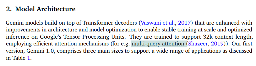
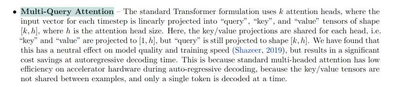
As a motivation, Gemini 1.0 was released on Dec 06 2023. Although they don’t disclose much about the architectural choices behind it, they made it clear that they’ve used MQA (pretty cool, huh?). As you see below, screen taken from the technical report.
Content:
- Batched Multi-Head Attention (MHA).
- Incremental Batched MHA.
- Multi-Query Attention (MQA).
- Incremental MQA.
TL;DR: Use only ONE key/value per multiple queries (i.e., drop the dim across the heads of K and V).
– Batched Multi-Head Attention (MHA, aka, Vanilla Attention):
- Notation:
model_size= dbatch_size= b (number of sequences)seq_len= nP_k, P_v, P_q: Projections matrics, with size \(hdk\), \(hdv\), and \(hdk\) respectively.- \(X, M\): Input and context matrices (sizes: \(bnd, bnd\))
- Careful, \(M\) is used with masking.
- Computing \(Q, K\) and \(V\):
Q=\(X\)@\(P_K\) (size: \(bhnk\))- Think of the dimension as follows: In each head \(h\), each token input \(n\) in seq \(b\), has a query \(q\) representation of dimension \(k\))
K=\(M\)@\(P_K\) (size: \(bhnk\))V=\(M\)@\(P_V\) (size: \(bhnk\), using \(k=v\))
- I’ll ignore the element-wise operations, as those do not change in neither MHA or MQA.
Here’s the provided script for completeness:
def MultiheadAttentionBatched(X, M, mask, P_q, P_k, P_v, P_o):
    """
    [...]
    P_q: a tensor with shape [h, d, k] # keep a look at the dim
    P_k: a tensor with shape [h, d, k] # keep a look at the dim
    P_v: a tensor with shape [h, d, v] # keep a look at the dim
    P_o: a tensor with shape [h, d, v]
    [...]
    """

    Q = tf.einsum("bnd,hdk->bhnk", X, P_q)
    K = tf.einsum("bmd,hdk->bhmk", M, P_k)
    V = tf.einsum("bmd,hdv->bhmv", M, P_v)
    [...]
    # the rest in un-changed in MQA.
– Performance analysis of Batched MHA:
- Total number of operations = \(\Theta(b n d^2)\), why \(\downarrow\)
- Let’s check \(Q\) for instance, we have
Q= \(X\)@\(P_K\) - \(X \rightarrow (bn \times d)\) and \(P_K \rightarrow (d \times hk)\)
- \(\implies Q\) takes \(\mathcal{O}(bn \times d \times hk) = \mathcal{O}(bn d^2)\) ops as \(hk = d\) (cute, innit?)
- Let’s check \(Q\) for instance, we have
- Total size of memory (to be accessed): \(b n d + b h n^2 + d^2\). Why \(\downarrow\)
- It’s just the size of the dimensions of all the actors:
- First term \(\rightarrow X, M, Q, K, V, O\) and, \(Y\)
- Second term for the point-wise ops \(\rightarrow\) logits, and softmax.
- Third term \(\rightarrow P_k, P_v, P_q\) and \(P_o\)
- It’s just the size of the dimensions of all the actors:
Ratio\(= \frac{\text{memory size}}{\text{# ops}} = \mathcal{O}(\frac{1}{k} + \frac{1}{bn})\)- The opposite of this ratio is known as Arithmetic Intensity (Not really but kinda related).
- Just keep in mind that it is necessary to keep this
ratio\(\ll 1\).
- Final note:
- This setting (Batched MHA) is what happens in training. We can see that as long as our \(nb\) is high, we are guarenteed to be in that
ratio\(\ll 1\) regime. Pretty cool, right?
- This setting (Batched MHA) is what happens in training. We can see that as long as our \(nb\) is high, we are guarenteed to be in that
– Incremental batched MHA (Inference):
Same as before, except here, we introduce and append the KV cache along the way.
def MHA(x, prev_K, prev_V, P_q, P_k, P_v, P_o):
    """Multi-Head Self-Attention (one step).

    Args:
    x: a tensor with shape [b, d]
    prev_K: a tensor with shape [b, h, m, k]
    prev_V: a tensor with shape [b, h, m, v]
    P_q: a tensor with shape [h, d, k]
    P_k: a tensor with shape [h, d, k]
    P_v: a tensor with shape [h, d, v]
    P_o: a tensor with shape [h, d, v]

    Returns:
    y: a tensor with shape [b, d]
    new_K: a tensor with shape [b, h, m+1, k]
    new_V: a tensor with shape [b, h, m+1, v]
    """
    q = tf.einsum("bd,hdk->bhk", x, P_q)
    new_K = tf.concat([prev_K, tf.expand_dims(
		tf.einsum("bd,hdk->bhk", M, P_k), axis=2)], axis=2)
    new_V = tf.concat([prev_V, tf.expand_dims(
		tf.einsum("bd,hdv->bhv", M, P_v), axis=2)], axis=2)
    logits = tf.einsum("bhk,bhmk->bhm", q, new_K)
    weights = tf.softmax(logits)
    o = tf.einsum("bhm,bhmv->bhv", weights, new_V)
    y = tf.einsum("bhv,hdv->bd", o, P_o)

    return y, new_K, new_V
– Analysis of Incremental batched MHA (Inference):
Similarily to the analysis in the batched MHA, we get for \(n\) generated tokens:
- #ops = \(\Theta (bnd^2)\)
- #memory = \(\Theta (b n^2 d + n d^2)\)
ratio= \(\mathcal{O}(\frac{n}{d} + \frac{1}{b})\)
Now, it’s tricky to push the ratio to be \(\ll 1\). We can’t just increase the batch size \(b\) as we are contsrained by the memory size. But also, when \(n \approx d\), memory bandwidth would be a bottleneck for performance. So, what do we do now? The author proposes, Multi-Query Attention (MQA). MQA radically removes the heads (h) dimension off \(K\) and \(V\).
– Multi Query Attention (MQA):
As you can see in the script below, MQA is literally MHA without the h dimension in K, and V.
def MultiQueryAttBatched(X, M, mask, P_q, P_k, P_v, P_o):
    """
    Args:
    [...]
    P_k: a tensor with shape [d, k]
    P_v: a tensor with shape [d, v]
    [...]
    """
    Q = tf.einsum("bnd,hdk->bhnk", X, P_q) #h is still there in the output dim
    K = tf.einsum("bmd,dk->bmk", M, P_k)   #h is dropped
    V = tf.einsum("bmd,dv->bmv", M, P_v) #h is dropped

    logits = tf.einsum("bhnk,bmk->bhnm", Q, K)
    # we recoved the same dim of the logits as the MHA,
    # everything is the same as MHA from now onwards.
    [...]
– Incremental MQA (Inference)
Differences in code are marked as #no h.
def MultiquerySelfAttentionIncremental(x, prev_K, prev_V, P_q, P_k, P_v, P_o):
    """
    Args:
    x: a tensor with shape [b, d]
    prev_K: a tensor with shape [b, m, k]  #no h
    prev_V: a tensor with shape [b, m, v] #no h
    P_q: a tensor with shape [h, d, k]
    P_k: a tensor with shape [d, k] #no h
    P_v: a tensor with shape [d, v] #no h
    P_o: a tensor with shape [h, d, v]
    [...]
    new_K: a tensor with shape [b, m+1, k] #no h
    new_V: a tensor with shape [b, m+1, v] #no h
    """
    q = tf.einsum("bd,hdk->bhk", x, P_q)
    K = tf.concat([prev_K, tf.expand_dims(tf.einsum("bd,dk->bk", M, P_k), axis=2)], axis=2)
    V = tf.concat([prev_V, tf.expand_dims(tf.einsum("bd,dv->bv", M, P_v), axis=2)], axis=2)

    logits = tf.einsum("bhk,bmk->bhm", q, K)
    # we revoved the dim `bhm`, the rest is same as before MHA.
    [...]
– Performance analysis for incremental MQA (Inference)
For \(n\) generations:
- #ops = \(\Theta (bnd^2)\)
- #memory = \(\Theta (b n^2 d + b n^2 k + n d^2)\)
ratio= \(\mathcal{O}(\frac{1}{d} + \frac{n}{dh} + \frac{1}{b})\)
Here we see that the problematic fraction \(\frac{n}{d}\) that we encountered in incremenral-MHA, is further devided by h… which helps tremendessly with performance.
I spent too much on this paper, here are some final notes:
- PaLM uses MQA. (see screenshot below from original paper, page: 5).
- One could argue that this improves throughput (we drop memory reqs, hence, we can increase
b?), rather than directly tackling latency. - MQA can lead to training instability in fine-tuning, especially with long input tasks. We notice some quality degradation and training instabiity with this method.
- Finally, to benefit from inference speed using MQA, models need to be trained on MQA, which is inconvenient. We would love a way to take advantage of MHA in training, but benefit from MQA in inference, and this is exactly what you get with Grouped Query Attention, presented next.
> Grouped Query Attention:
- This Paper provides two contributions:
- A way to uptrain models with MHA into MQA.
- \(\implies\) no need to train models from the start with MQA, you can just use MHA then switch in inference to MQA.
- A generalization to MQA.
- A way to uptrain models with MHA into MQA.
- Note: This switch in training/architecture from MHA \(\rightarrow\) MHA is a Procedure known in the literature as Upcycling/Uptraining (Check this paper for detais):
– Uptrainig from MHA to MQA happens in 2 steps:
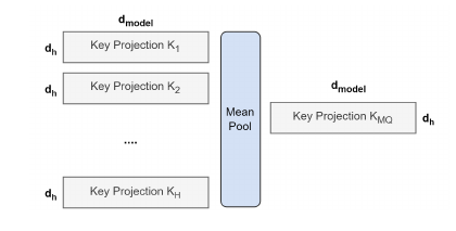
- Convert checkpoint (snapshot of weights)
- Key and Value projection matrices are mean pooled into a single (see screen 2 below).
- Additional pre-training on a small percentage \(\alpha\) to adapt to the new structure.
- They uptrained with \(\alpha = 0.05\) of the original pre-training steps of T5.
Final interesting takes:
- They do not evaluate on classification benchmarks, as GLUE (reason: Autoreg. inference is weak/less applicable to these tasks).
- Uptraining for 5% is optimal for both MQA and GQA, pushing it higher (10%) did not help much.
Coincid.. Gemini just dropped, and one of the few details about the architeture is that they used MQA… , pretty cool, huh??
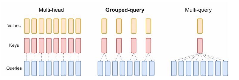
– Grouped Query Attention:
Instead of all queries of an attention layer having the same key/value (MQA), we group queries into sub-groups that share the key/value (Check screen 1 below).
– Final notes:
GQA » Increase in inference speed && Reduces memory requirement during decoding. » Higher batch size » Higher throughput
> Sliding Window Attention:
TODO
Relevent literature: Longformer, Sparse Transformers.
Vanilla attention scales quadratically with long sequences (Quick Why: with each input of the sequence (length n), you compute n weight/ reformulate this.)
– Longformer attention combines:
- Windowed attention (local) \(\rightarrow\) build a contextualized representation.
- End task global attention \(\rightarrow\) build full sequence representations for prediction.
Attention pattern:
- Sliding windon of fixed size around each token \(\implies\) attention matrix is sparsified.
- Q: Is it literally masked? Q = Q’ x Mask ? Yes/No.
- x
– Sparse Transformers:
TL;DR: Add more sparsity to you attention weights. By shortening your attention span. Instead of accessing all you past, access only up to a window \(W\) (not really, they defind a pattern of “attendence”, will get to it later, the change the usual mask).
Section 4.2 is so well written, that I’m technically going to be re-writing it.
Vanilla attention (this is a mathpix test, looking fine on markdown so far):
\[\begin{gathered} \operatorname{Attend}(X, S)=\left(a\left(\mathbf{x}_i, S_i\right)\right)_{i \in\{1, \ldots, n\}} \\ a\left(\mathbf{x}_i, S_i\right)=\operatorname{softmax}\left(\frac{\left(W_q \mathbf{x}_i\right) K_{S_i}^T}{\sqrt{d}}\right) V_{S_i} \\ K_{S_i}=\left(W_k \mathbf{x}_j\right)_{j \in S_i} \quad V_{S_i}=\left(W_v \mathbf{x}_j\right)_{j \in S_i} \end{gathered}\]> Flash Attention:
TODO
This 34 pages idea, wins the price of “Minimum innovation, maximum results– Ilya Sutskever”
One of the ideas: Basically, instead of moving KV’s around, just recompute them at backprop.
Why: Compute capabilities on GPUs is 2 orders of magnitude higher than memory. recompute is easy, moving data and storing it in GPUs is hard. Q: I thought OpenAI was already doing this, in their 2019 paper. Investigate this!!
> Notes on Mistral 7B:
The ratio of \(\frac{\text{ideas}}{\text{pages}}\) in the Mistral 7B is too high. It combines efficiently all the techniques that are mentioned above. Additionally, they use:
- Rolling buffer Cache:
Set the cache size to a value \(W\), and store the keys and values at step \(i\) at position \(i \equiv W\) (modulo) \(\implies\) starting from step \(W\), cache get overwritten with new values.
Why is it fine to do so: because we add positional encoding before, so it doesn’t really matter where do you store, attention is a “set” operation.
- Pre-fill and Chunking:
I don’t get this yet. Check it later!
(Of course it’s related to KV cache.)
(pre-fill, is computing the KV of the prompt, which is already available in advance, hence we can chunk it, etc.)
(Chunking: Split the prompt size in chunks of size \(W\) (window size of the attention) » Then what?)
> Speculative decoding:
– Quick Terminology:
- Target model: A big model (the one we want to eventually optimize), e.g., Llama 70B
- Draft model: A small/fast model, e.g., Llama 7B
– Main obsevation:
- Time wise, scoring a short continuation of the draft model \(\approx\) Generating 1 token by target model.
– Main idea:
- Generate tokens with draft model and verify along the way with target model, and correct when necessary.
Autoregressive sampling is memory bandwidth bound:
- Mainly becasue we load huge parameters, and construct a huge KV cache
Latency\(\displaystyle \propto\)params_sizeXtransformer_memory_size- Looks cute, but why?
- With longer context, your KV cache takes over, and optimizing compute doesn’t cut it anymore. I.e., you’re stuck in memory bound regime (Check the original “Making DL go brrr” blog for more.).
Why is scroring a draft continuation has \(\sim\) latency to generating a token.
TODO
- Input: Prompt \([x_1, \dots, x_{T-1}]\)
- Task 1: Generate the next token \(x_{T}\)
- Task 2: Verify is some token \(q_{T}\) is a plausible generation.
Imagine having a draft model (typically fast/small), and a target model, typically big (think of the former as a Llama 7B, and the latter as a Llama 70B).
Speculative decoding in a nutshell:
- Generate a sequence of \(K\) (~ 4/5) tokens using the draft model.
- Scoring the the sequence using the target model.
- Accept/Reject the proposed sequence using a rejection sampling inspired technique, that hopefully recovers the target model output distribution.
Useful links:
TODO:
- verify the links/ in the contents.
- Proof-Check MQA.
- Have a sync’ed way of listing the references for each section.
- Check, and update.